Example 1
{{SimInitialize-nav}} Next, verify that the piston is not in motion. The piston is not in motion if the piston button is labeled "Release Piston". If the piston button is labeled "Hold piston", push that button.
Set the initial conditions (Any parameter not mentioned should be left at the default):
- Use a simulation in 3D space
- Set Temperature : Adiabatic
- Pressure : 500
- Number of Molecules : 100 (this is not editable)
- Intermolecular Potential : Ideal gas
Start the simulation by pushing the start button and then pushing the piston button. Observe the fluctuations of the piston (on the piston-cylinder graphic) as it falls under the influence of the imposed (500 bar) pressure and rises in response to the collisions with the molecules. Note the fluctuations in the values given in the density boxes and the temperature boxes. Next, Increase the pressure to 1000 bar by moving the pressure slider to the right, and observe the decrease in the volume in the animation and the rise in density reported in the density boxes.
Click on the tab labeled "Plots". You should now see graphs that look something like the following (NOTE : If enough time has passed since the pressure slider was changed to 1000, the transition will not be seen on the graph as that data has already scrolled off the graph) :
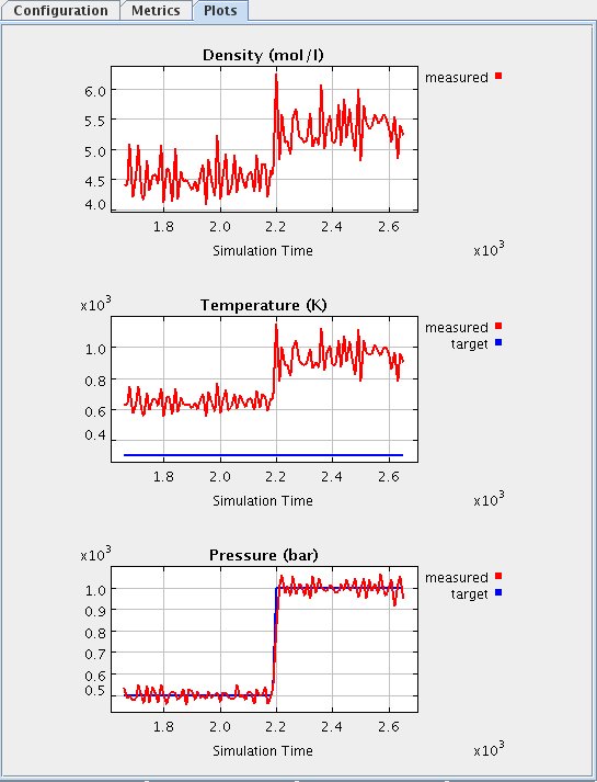
This graph shows a recent history of the values of several of the system properties. The graph may not show all of the data since the simulation was started. Once the maximum amount of data is displayed on the graph, old data will be scrolled off the graph to the left as new data is added to the right. Four properties are shown.
- The measured density of the system is shown on the top plot (density graph). The plot shows how the density responded to the pressure increase, clearly increasing at the point when the pressure was raised (around 2200 picoseconds as shown on X axis).
- The middle plot (temperature graph) show the temperature of the system. The plot shows how the temperature responded to the pressure increase, clearly increasing at the point when the pressure was raised (around 2200 picoseconds as shown on X axis).
- The bottom plot (pressure graph) shows the pressure measured on the piston, due to collisions with the molecules. The measured pressure curve (in red) shadows the target pressure (in blue), showing that the piston moves to a point where the external and internal pressure forces balance.
Play around with the pressure slider, taking it down to 100 bar, and later back up to 500 or 1000, and observe the response of the system by looking both at the piston-cylinder graphic behavior and the graphs.